Gradient Descent Algorithms! Ready steady Go!
· 4 min read
Optimization, Gradient Descent
Two years back I went through this paper — An overview of gradient descent optimization algorithms by Sebastian Ruder. But apart from the takeaway that "Momentum helps escape the local minimum", I had forgotten everything. So I decided to take this paper again and work myself through various algorithms.
Gradient Descent is an optimization technique that iteratively updates the parameters of the neural network. There are family of algorithms and types of Gradient descent techniques. On one hand you can divide the algorithms into three types depending on how much data was used to update the parameters. The methods are — Batch Gradient Descent, MiniBatch Gradient Descent, and Stochastic Gradient Descent. The other way of characterizing the algorithms is coming up with ways that solves the challenges of the Vanilla Mini-Batch gradient descent.
Btw, the vanilla mini-batch gradient descent looks like this — $$ \theta = \theta - \eta \cdot \nabla_{\theta} J(\theta; x^{(i:i+n)}; y^{(i:i+n)}) $$ I often get confused between the use of $\theta$ in $\nabla_\theta$ and $J(\theta)$. Here $\nabla_\theta$ means taking the gradient w.r.t parameters $\theta$. And $J(\theta)$ means taking the gradient of the parameters like weights and biases and not the input of the network. Hope this clears the confusion.
Note — Mini-batch gradient descent is typically the algorithm of choice when training a neural network and the term SGD usually is employed also when mini-batches are used.
As stated above, the challenges with vanilla gradient descent are —
- Choosing a proper learning rate can be difficult.
- The learning rate schedules must be defined in advance, and are unable to adapt to a dataset's characteristics.
- The same learning rate gets applied to all parameters — e.g. for both sparse data and features with different frequencies(explained below) the same rate gets applied.
- Avoiding getting trapped/slowed down by numerous suboptimal local optima/characteristics of the non-convex error function like saddle point, plateaus, ravines, etc.
- Batch Gradient Descent cannot naturally learn from new examples one at a time as they arrive. It typically needs to process the entire training dataset to calculate each gradient update.
Sparse data — There are 100,00 words in the vocabulary and we are having a document with 300 unique words. Thus, 999,700 are absent from that document. If you were to represent this as a matrix, with putting 1 where a word was present, then for a document most values would be zero.
| Documents | apple | cricket | football | science | ... | zebra |
|---|---|---|---|---|---|---|
| Document 1 | 1 | 0 | 0 | 1 | ... | 0 |
| Document 2 | 0 | 1 | 1 | 0 | ... | 0 |
Features with different frequencies — Let's say we have 1 million such documents. Now count the frequencies for each word across documents. The frequencies would look probably like —
| Feature | Frequency | Frequency type |
|---|---|---|
| apple | 100,000 | very common |
| cricket | 150,000 | very common |
| science | 50,000 | common |
| zebra | 350 | rare |
The problem is the very common feature will get updated several times, and the rare feature will not get enough chances to update well. For this, we must use a Parameter specific weighted update methods (Adaptive Gradient Descent Methods like — Adagrad, Adadelta, Adam, etc). But we are running ahead of ourselves for now.
Momentum — Enter the first SGD variant
SGD has trouble navigating ravines i.e. areas where the surface curves much more steeply in one dimension than in another, which are common around local optima.
SGD oscillates across the slopes of the ravine while only making hesitant progress along the bottom towards the local optimum.
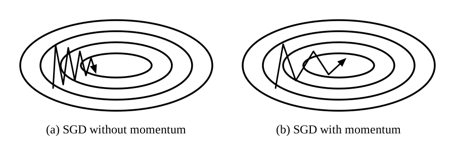
Momentum is a method that helps accelerate SGD in the relevant direction and dampens oscillation. The update rule is broken down into two steps: $$ v_t = \gamma v_{t-1} + \eta\nabla_\theta J(\theta) \ \theta = \theta - v_t $$ To develop the intuition for this formula, I like to think in the reverse order. Here $v_t$ must be of the same units as $\nabla_\theta J(\theta)$ — otherwise how would we add them together. $\gamma$ and $\eta$ are just some constants that defines how much to quantify each value.